Sampling, integration and volume computation in R

In this blog post we will compare several R packages with volesti. volesti is a C++ library for volume approximation and sampling of convex bodies (e.g. polytopes) with an R interface hosted on CRAN. volesti is part of the GeomScale project.

The goal of this blog post is to show that volesti is the most efficient choice, among R packages in a number of high dimensional computational tasks, namely:

• to sample from the uniform or a restricted Gaussian distribution over a polytope,
• to estimate the volume of a polytope,
• to estimate the integral of a multivariate function over a convex polytope.

In particular, we will compare volesti with:

1. hitandrun, a package that uses Hit-and-Run algorithm to sample uniformly from a convex polytope.
2. restrictedMVN, a package that uses Gibbs sampler for a multivariate normal restricted in a convex polytope.
3. tmg, a package that uses exact Hamiltonian Monte Carlo with boundary reflections to sample from a a multivariate normal restricted in a convex polytope.
4. geometry, the R interface of C++ library qhull. It uses a deterministic algorithm to compute the volume of a convex polytope.
5. SimplicialCubature, a package to integrate functions over m-dimensional simplices in n-dimensional Euclidean space.

To run the following scripts we will need to import the following R packages,

library(volesti)
library(hitandrun)
library(geometry)
library(SimplicialCubature)
library(ggplot2)
library(plotly) 
library(rgl)
library(coda)
library(Rfast)
library(pracma)

Note that we use R 3.6.3 throughout the blog post.

Comparison with hitandrun

Uniform sampling from a convex polytope is of special interest in several applications. For example in analyzing metabolic networks or explore the space of portfolios in a stock market.

hitandrun takes as input the linear constraints that define a bounded convex p olytope and the number of uniformly distributed points we wish to generate together with some additional parameters (e.g. thinning of the chain).

The following script first samples 1000 points from the 100-dimensional hypercube \([-1,1]^{100}\) using both hitandrun and volesti. Then, measures the performance of each package defined as the number of effective sample size (ESS) per second.

d = 100
P = gen_cube(d, 'H')

constr = list("constr" = P@A, "dir" = rep("<=", 2 * d), "rhs" = P@b)

time1 = system.time({ samples1 = t(hitandrun::hitandrun(constr = constr, 
    	n.samples = 1000, thin = 1)) })

time2 = system.time({ samples2 = sample_points(P, random_walk = list(
    	"walk" = "RDHR", "walk_length" = 1, "seed" = 5), n = 1000) })                
cat(min(coda::effectiveSize(t(samples1))) / time1[3],
    min(coda::effectiveSize(t(samples2))) / time2[3])

The ESS of an autocorrelated sample, generated by a Markov Chain Monte Carlo sampling algorithm, is the number of independent samples that it is equivalent to. For more information about ESS you can read this paper. To estimate the effective sample size we use the package coda.

The output of the above script,

0.02818878 74.18608

shows that the performance of volesti is ~2500 times faster than hitandrun.

The following R script generates a random polytope for each dimension and samples 10000 points (walk length = 5) with both packages.

for (d in seq(from = 10, to = 100, by = 10)) {
  
  P = gen_cube(d, 'H')
  tim = system.time({ sample_points(P, n = 10000, random_walk = list(
      "walk" = "RDHR", "walk_length"=5)) })
  
  constr <- list(constr = P$A, dir=rep('<=', 2*d), rhs=P$b)
  tim = system.time({ hitandrun::hitandrun(constr, n.samples = 10000, thin=5) })
}

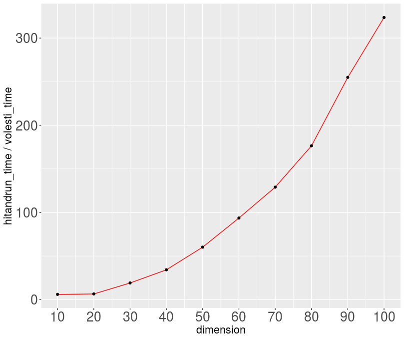
The following Table reports the run-times.

dimension	volesti time	hitandrun time
10	0.017	0.102
20	0.024	0.157
30	0.031	0.593
40	0.043	1.471
50	0.055	3.311
60	0.069	6.460
70	0.089	11.481
80	0.108	19.056
90	0.132	33.651
100	0.156	50.482

The following figure illustrates the asymptotic in the dimension difference in run-time between volesti and hitandrun.

Comparison with restrictedMVN and tmg

In many Bayesian models the posterior distribution is a multivariate Gaussian distribution restricted to a specific domain. For more details on Bayesian inference you can read the Wikipedia page.

We illustrate the efficiency of volesti for the case of the truncation being the canonical simplex,

$$\Delta^n =\{ x\in\mathbb{R}^n\ |\ x_i\geq 0,\ \sum_ix_i=1 \}.$$

This case is of special interest and typically occurs whenever the unknown parameters can be interpreted as fractions or probabilities. Thus, it appears naturally in many important applications.

In our example we first generate a random 100-dimensional positive definite matrix. Then, we sample from the multivariate Gaussian distribution with that covariance matrix and mode on the center of the canonical simplex. To achieve this goal we first apply all the necessary linear transformations to both the probability density function and the canonical simplex. Last, we sample from the standard Gaussian distribution restricted to the computed full dimensional simplex and we apply the inverse transformations to obtain a sample in the initial space.

d = 100
S = matrix( rnorm(d*d,mean=0,sd=1), d, d) #random covariance matrix 
S = S %*% t(S)
shift = rep(1/d, d)
A = -diag(d)
b = rep(0,d)
b = b - A %*% shift
Aeq = t(as.matrix(rep(1,d), 10,1))
N = pracma::nullspace(Aeq)       
A = A %*% N #transform the truncation into a full dimensional polytope
S = t(N) %*% S %*% N
A = A %*% t(chol(S)) #Cholesky decomposition to transform to the standard Gaussian
P = Hpolytope(A=A, b=as.numeric(b)) #new truncation

Now we use volesti, tmg and restrictedMVN to sample,

time1 = system.time({samples1 = sample_points(P, n = 100000, random_walk = 
    list("walk"="CDHR", "burn-in"=1000, "starting_point" = rep(0, d-1), "seed" = 
    127), distribution = list("density" = "gaussian", "mode" = rep(0, d-1))) })

# tmg does not terminate
time2 = system.time({samples2 = tmg::rtmg(n = 100000, M = diag(d-1), r = 
    rep(0, d-1), initial = rep(0, d-1), P@A, P@b, q = NULL, burn.in = 1000) })            

time3 = system.time({samples3 = restrictedMVN::sample_from_constraints(
    linear_part = A, offset= b, mean_param = rep(0,d-1), covariance = diag(d-1), 
    initial_point = inner_ball(P)[1:(d-1)], ndraw=100000, burnin=1000) })   
                  
# print the performance (effective sample size over time)
cat(min(coda::effectiveSize(t(samples1))) / time1[3],
    min(coda::effectiveSize(samples3)) / time3[3])

the output of the script,

30.3589 3.936369 

Now we can apply the inverse transformation,

samples_initial_space = N %*% samples1 + 
   kronecker(matrix(1, 1, 100000), matrix(shift, ncol = 1))

Allow us to conclude that volesti is one order of magnitude faster than restrictedMVN for computing a sample of similar quality. Unfortunately, tmg failed to terminate in our setup.

Comparison with geometry

Next comparison is about volume computation of convex polytopes. It will help us to understand the need of randomized computation in high dimensions implemented in volesti.

geometry is considered as the state-of-the-art volume computation package in R today but also on of the most efficient package for volume computation in general. To compute the volume geometry deterministically build a triangulation of the input polytope that can grow exponentially with the dimension. Thus, inevitably, such an implementaion will end out of memory at some point. For more details about the volume algorithms in geometry you can read qhull documentaion.

First we make the comparison in dimension 15,

P = gen_rand_vpoly(15, 30, generator = list("body" = "cube", "seed" = 1729))

time1 = system.time({geom_values = try(geometry::convhulln(P@V, options =
    'FA'))})

time2 = system.time({vol2 = volume(P, settings = list("algorithm" = "CB",
    "random_walk" = "BiW", "seed" = 127)) })

cat(time1[3], time2[3], geom_values$vol, vol2, abs(geom_values$vol - vol2) 
    / geom_values$vol)

In this dimension, using geometry is more efficient than volesti. This happens because the dimension 15 is a relatively small dimension and the geometry’s run-time does not yet explodes. Let us continue with an example in 20 dimensions to see how this picture changes.

P = gen_rand_vpoly(20, 40, generator = list("body" =  "cube", "seed" = 1729))

time1 = system.time({geom_values = geometry::convhulln(P@V, options = 'FA')})

and then, we have a run-time error,

QH6082 qhull error (qh_memalloc): insufficient memory to allocate 1329542232 bytes

Which means that geometry fails to compute this volume due to insufficient memory allocation. On the other hand, the same instance can be approximated by volesti in a few seconds,

time2 = system.time({ vol2 = volume(P, settings = list( "seed" = 5)) })

cat(time2[3], vol2)

The output is,

23.888 2.673747398e-07

Hence volesti is the only way to estimate the volume of high dimensional polytopes in R.

Comparison with SimplicialCubature

Computing the integral of a function over a convex set (here, convex polytope) is one of the oldest mathematical problems and is important for many scientific applications.

In R the package SimplicialCubature computes multivariate integrals over simplices. For the general case of a polytope one way to go is to compute the Delaunay triangulation with package geometry and then use the package SimplicialCubature to sum the values of all the integrals over the simplices of the triangulation.

On the other hand, volesti can be used to approximate the value of such an integral by a simple Markov Chain Monte Carlo integration method, which employs the volume of the polytope, say P, and a uniform sample in P.

In particular, if we want to compute

$$I = \int_P f(x)dx .$$

we sample N uniformly distributed points from P and,

$$I \approx vol(P) (1/N) \sum_{i} f(x_i).$$

The following script generates random polytopes for dimensions d = 5, 10, 15, 20 and defines the integrand function f. Then computes the exact value of the integral of f over each polytope using SimplicialCubature and geometry. In the sequel, we approximate that integral with volesti.

for (d in seq(from = 5, to = 20, by = 5)) {
       P = gen_rand_vpoly(d, 2 * d, generator = list("seed" = 127))
       tim1 = system.time({ 
           triang = try(geometry::delaunayn(P@V))
           f = function(x) { sum(x^2) + (2 * x[1]^2 + x[2] + x[3]) }
           I1 = 0
           for (i in 1:dim(triang)[1]) {
               I1 = I1 + SimplicialCubature::adaptIntegrateSimplex(f, 
               t(P@V[triang[i,], ]))$integral
           } 
    })
    tim2 = system.time({ 
        num_of_points = 5000
        points = sample_points(P, random_walk = list("walk" = "BiW", 
            "walk_length" = 1, "seed" = 5), n = num_of_points)
        int = 0
        for (i in 1:num_of_points){
            int = int + f(points[, i])
        }
        V = volume(P, settings = list("error" = 0.05, "seed" = 5))
        I2 = (int * V) / num_of_points 
    })
    cat(d, I1, I2, abs(I1 - I2) / I1, tim1[3], tim2[3], "\n")
   }

and we obtain the following results,

5   0.02738404    0.02446581    0.1065667   0.023    3.983 
10  3.224286e-06  3.204522e-06  0.00612976  3.562    11.95 
15  4.504834e-11  4.867341e-11  0.08047068  471.479  33.256 
20  halts         1.140189e-16  -           -        64.058

Notice that the pattern is similar to volume computation. For d = 5, 10 the exact computation with SimplicialCubature is faster than the approximate with volesti. For d = 15, volesti is 13 times faster and for d = 20 the exact approach halts while volesti returns an estimation in about a minute. The reason is that the run-times of both the computation of the Delaunay triangulation with package geometry and the exact computation of the integral with SimplicialCubature grow exponentially with the dimension. On the other hand, the run-time of volesti grows polynomially with the dimension.

Conclusions

In this blog post we compared volesti with five R packages in certain challenging computational problems:

1. sampling from polytope,
2. volume computation of polytopes and
3. computing the integral of a function over a polytope.

We found volesti faster in all cases as the dimension grows. Especially in the cases where the exact algorithms halt (for dimensions larger than 20), volesti takes a few seconds or minutes to estimate the desired quantity. The reasons behind this success is the efficient geometric random walks implemented in volesti and the fast randomized approximation algorithms for volume computation.

Computational details

The results in this blog were obtained using R 3.4.4 and R 3.6.3 and volesti 1.1.2. The versions of the imported by volesti packages are stats 3.4.4 and methods 3.4.4; of the linked by volesti packages, Rcpp 1.0.3, BH 1.69.0.1, RcppEigen 0.3.3.7.0, and the suggested package testthat 2.0.1. For comparison with volesti and plots, geometry 0.4.5, hitandrun 0.5.5, SimplicialCubature 1.2, ggplot2 3.1.0, plotly 4.8.0, rgl 0.100.50, coda 0.19.4. All packages used are available from CRAN.

All computations were performed on a PC with Intel Pentium(R) CPU G4400 @ 3.30GHz x 2 CPU, 16GB RAM.